Using PowerSwift™ 2.1
PowerSwift™ is simple to use. Screen shots of a sample design are shown below for reference.
The present version of PowerSwift™ is a Windows application, not a web service. Tutorial updated 11-6-11
COPYRIGHT ™ 2012 Photovoltaic Resources International Corp.
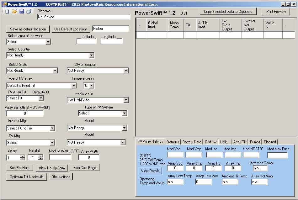
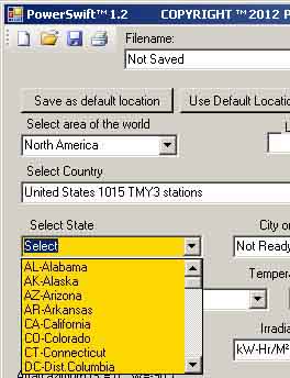
The starting screen is shown above. The first step is to specify a location for sunshine and temperature. PowerSwift™ has data available for most areas of the world. USA data has additional temperature extremes added for design of utility interactive inverter systems.The location can be selected as either the previously saved specific default, or selected by 'Area of the World'/'Country'/'State'/'City or Location'. Owners of the earlier PVCAD versions can use their existing data files. The Open File icon in the upper left is used to reload saved designs.
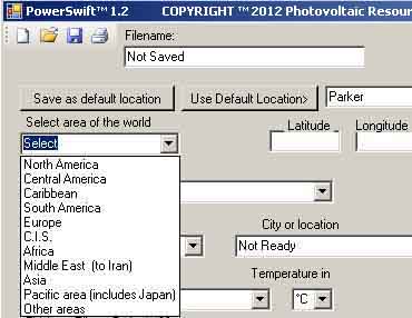 Then select
file>
Then select
file> 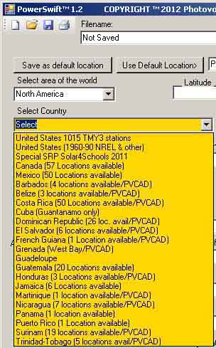
 ------------------>
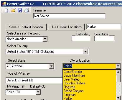
The 'United States 1015 TMY3 stations' file has 1015 locations with the additional temperature data for grid interactive inverters. Notice that the background color changes in the next logical entry box. This example has selected the data from Sky Harbor airport in Phoenix, Arizona. This site can be saved as the default location by clicking on 'Save as default location'. Future plans are to supplement this procedure with state maps showing the location of data sites.
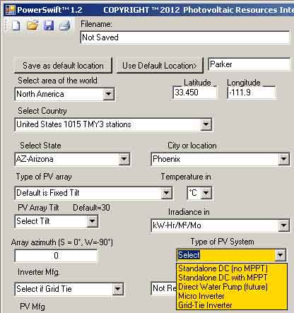
Next the user should select the type of PV system, the present choices are:
Standalone DC system without a Maximum Power Point Tracker.
Standalone DC system with a Maximum Power Point Tracker
Micro Inverter (features more detailed AC wiring design)
Grid-Tie Inverter (This will be used for the introduction.)
There will be future options such as direct connected DC water pumps that will require specific design files (Sunpumps).
If Standalone or water pumps are selected, the inverter selection boxes will not show.
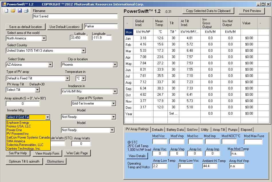
Note that the performance grid now shows, but is incomplete.
Next, select the Inverter Manufacturer from the drop-down list.
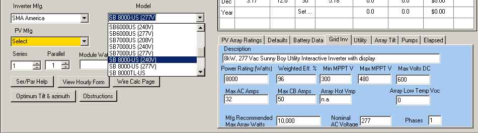
Select the inverter/nominal voltage from the drop-down list. Note that the 'Grid Inv' tab in the blue tabbed data area is selected for display. The inverter can be reselected at any time if a change is necessary.
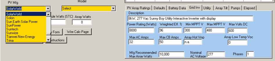
Note the inverter data that has been loaded. Next Select the 'PV Mfg' from the drop-down list.
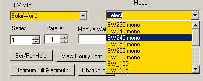
Select the desired PV module. It can be changed later if need be.
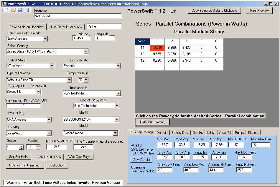
The array starts as one PV module. Click on the 'PV Array Ratings' tab to display the array data. The temperature related variables are calculated based on the site data and the module data. Note the Pop-Up with the allowable Series-Parallel combinations based on the module voltages, ambient temperatures and inverter maximum recommended power. The red combination exceed the recommended maximum power. The user can click on the desired Series-Parallel combination or use the 'Series' and 'Parallel' selection boxes to increase the array size. Click on the 'Grid Inv' tab for the next step.
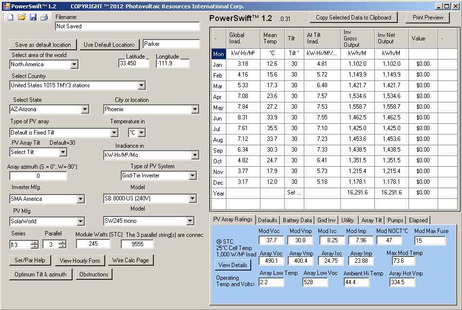
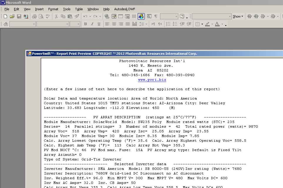
The above image shows a suitable design. The Value $ column is zero because the Utility rate schedules needs to be selected. There are presently Arizona rates available. Users can construct other rates by following the examples. Click the 'Utility' tab. Note the buttons 'View Hourly Form' and 'Wire Calc Page' for later use.
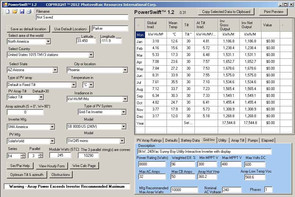
Note the warning that appears above as the result of increasing the Series modules to 14. As the array is adjusted, the result is compared to the inverter requirements. There are also warnings if 'Array Hot Vmp' is below the 'Min MPPT V' specification of the inverter. There will be warnings for voltage and power being too high.
 --->
--->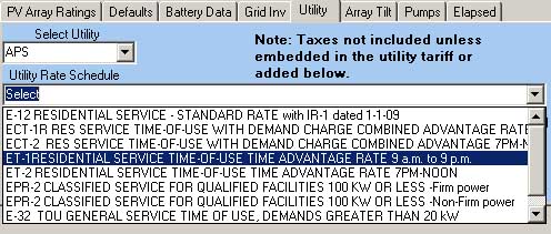
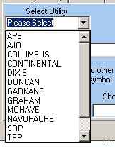
The available utility rates are shown above. Select the desired rate. The value of the system output is calculated by applying the rate to each hour of a typical year, adjusting for the weekends and holidays. Use Excel to look at the rate schedules and to make other schedules.
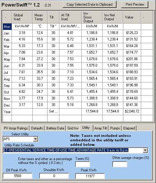
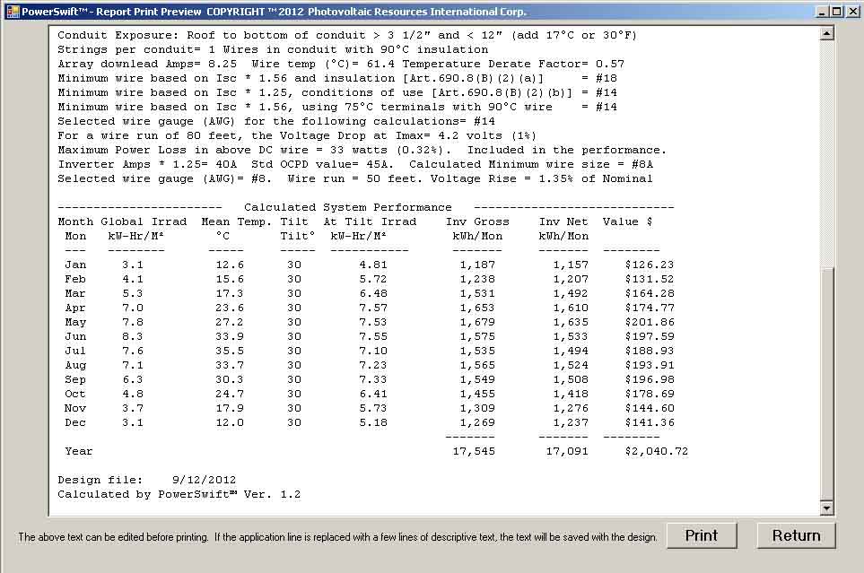
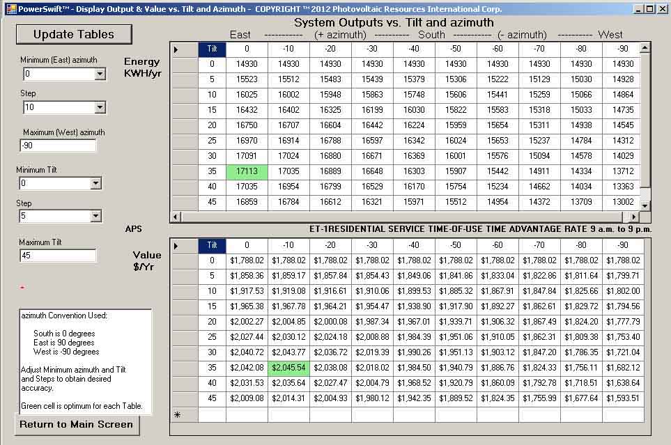
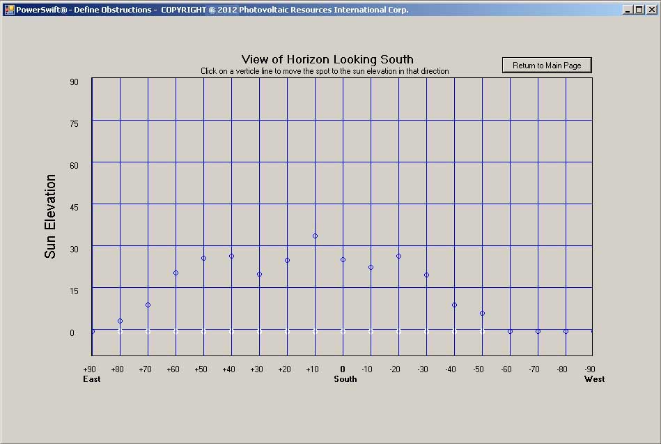
The above shows the value of the electrical output for the selected rate schedule. This is for a South facing array at 30° tilt. Adjust the tilt and azimuth (non-south direction, East =90, etc.). The performance will change in response.
If other than the 5-degree steps are needed, or there will be seasonal changes, the tilt values in the performance Table can be changed (Edit the values, then click on the cell with 'Set Tilt').
The data in the Performance Table can be placed on the Windows clipboard for use in other applications such as spreadsheets and documents. (Selected the desired range with a mouse to highlight the desired data, then click the button ot the top labeled 'Copy Selected Data to Clipboard' ). Before doing this, look at the printed report as that data can also be copied, but not as cells.
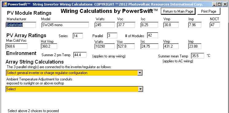
Clicking on the 'Wire Calc Page' button displays the above page as a guide to selecting the correct wire sizes and understanding the effect of decisions such as height of the roof mounted conduits (per 2011 version of the National Electrical Code).
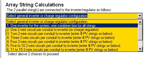
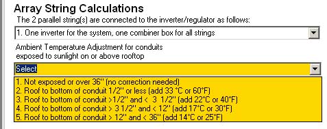
The yellow selections must be made to proceed.
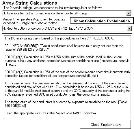
Clicking on the 'Show Calculation Explaination' button will pop-up the above descriptions of the calculations.
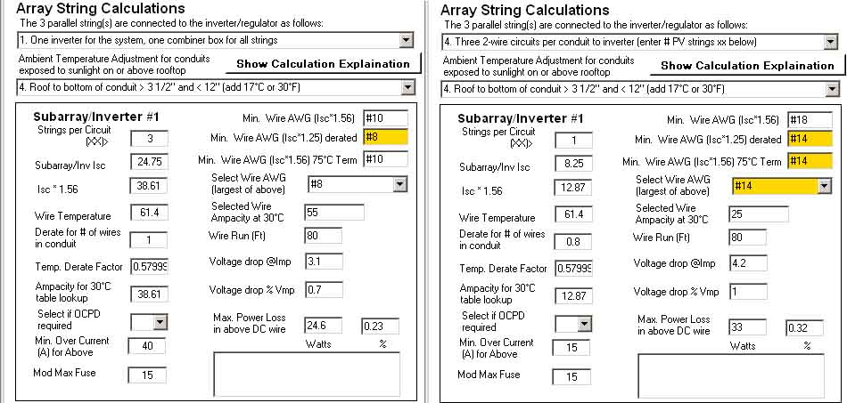
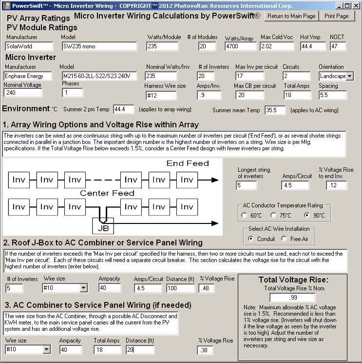
The above shows two possibilities for the illustrated design. The left image uses a combiner box to allow a single pair of downlead wires, and the right image has two modules strings in the same conduit. The fuse data is significant if more than two module strings are in parallel, see Article 690 of the NEC. #10 wire was selected for the right image because the #12 wire would not be protected by a 15A fuse at the working temperature of the wire. The voltage drop and power loss is not significant in this system design.
Note that there are three Minimum wire size recommendations, based on the three requirements of the NEC. Pick the heaviest wire size.
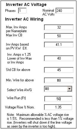
The AC wiring is important because there are limits to the acceptable Voltage Rise in the wiring due to wire resistance. Most inverter manufacturers recommend that this be less than 1%, otherwise the inverter may trip off due to sensing utility voltage that are out of the allowable range. In the example above, if #8 wire were used the limit for wire length is 36 feet. If a 3-phase inverter is used the values are adjusted accordinly. If single phase inverters are used at 208 volts or 277 volts, a warning about 3-phase currents appears.
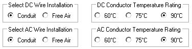
Note that while the default is 90°C rated wire in conduit, wire in free air and lower rated wire can be specified.
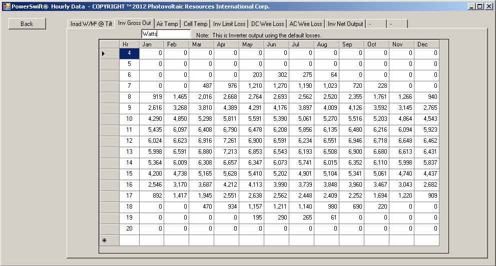
Clicking the 'View Hourly Form' button on the main page allows the user to view the hourly data for reference. The hourly output of the inverter is shown above. Note the other tabs for additional data.
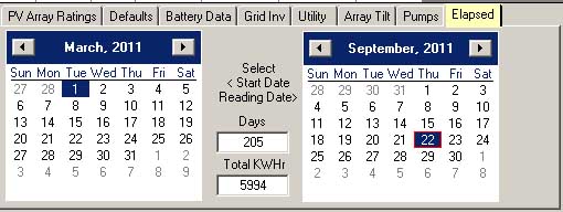
One feature of PowerSwift™ is the calculation of expected system output over a specific date range. Handy for checking on system performance. Obsolete PV module models will be maintained in the database to support checking on older systems.